9  Mixing

# Access custom defined functions
targets::tar_source("../R_functions")

make_plotdata_racegender_mixing_matrix() |>
  plot_matrix_mixing() +
  scale_fill_mpxnyc_gradient() +
  scale_color_mpxnyc_gradient() +
  theme_mpxnyc_mixing()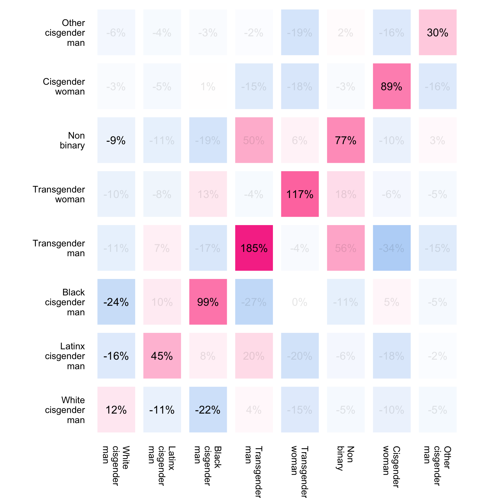

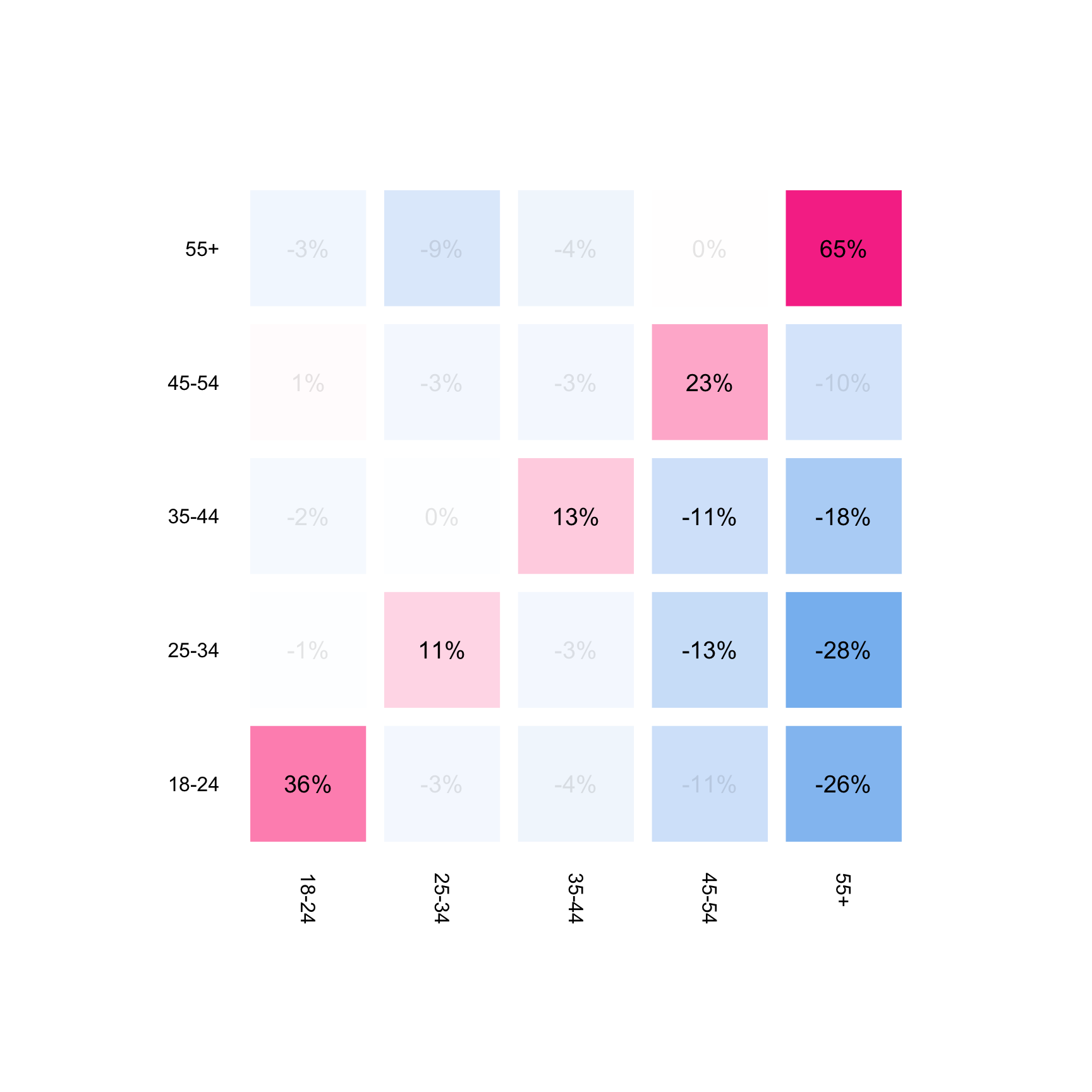
Figure 9.1: Spatial mixing matrix by race and gender.

Patterns of mixing reveal how social worlds overlapped—and where they stayed distinct—within queer and trans New York. Using spatial mixing coefficients, we measured the degree to which participants who shared certain characteristics (such as race, gender, sexual orientation, or age) tended to live or play in the same neighborhoods.

Across all categories, participants showed spatial homophily—people were more likely to live or go out in community districts where others shared their demographic traits. Yet the pattern was not uniform.Latinx cisgender men, Black cisgender men and non-binary participants tended to visit or reside in different neighborhoods than white cisgender men, indicating parallel but distinct social geographies.

make_plotdata_sexorientation_mixing_matrix() |>
  plot_matrix_mixing() +
  scale_fill_mpxnyc_gradient() +
  scale_color_mpxnyc_gradient() +
  theme_mpxnyc_mixing(
    plot.margin = ggplot2::unit(10*c(10,10,10,10), "pt")
    ) 

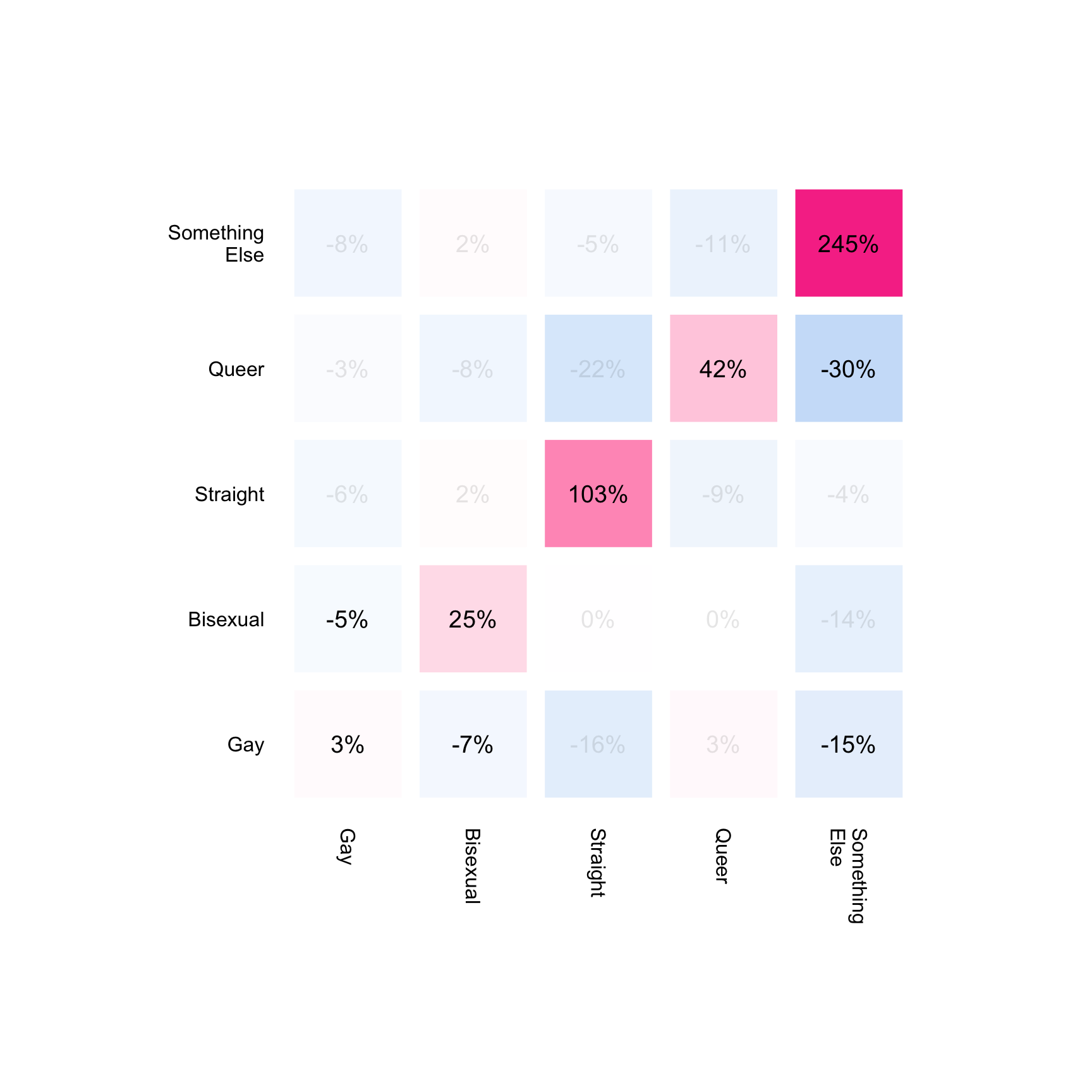
Figure 9.2: Spatial mixing matrix by sexual orientation

When we examine sexual orientation, gay-identified participants clustered in neighborhoods where bisexual participants were less present—and this groups, in turn, was less present in gay-leaning clusters of neighborhoods. These mirrored preferences underscore how social identity, geography, and nightlife intertwine to shape opportunity for connection—and risk for infection.

make_plotdata_age_mixing_matrix() |>
  plot_matrix_mixing() +
  scale_fill_mpxnyc_gradient() +
  scale_color_mpxnyc_gradient() +
  theme_mpxnyc_mixing(
    plot.margin = ggplot2::unit(10*c(10,10,10,10), "pt")
    ) 

Figure 9.3: Spatial mixing matrix by age

In terms of age, 25 to 44 year olds tended to be in different districts than those over 45. In addition, 18-24 year olds tended to be in different districts than those over 55.

plot_icon(icon_name = "bear", color = "light_brown", shape = 8)