Code
plot_icon(icon_name = "devil", color = "light_purple", shape = 16, alpha = 0, size = 100, image_size = 0.2)
We describe the main data object of the SSNAC framework: the person-place graph. We also define some useful statistics for the descriptive analysis.
plot_icon(icon_name = "devil", color = "light_purple", shape = 16, alpha = 0, size = 100, image_size = 0.2)
You are town epidemiologist in a town of 8000 people who live and work across 5 communities. You hear news of a novel human transmitted infection coming to the town. You decide to map the spatial and sexual networks of the townspeople to prepare for a response to the new infection. You take a random sample of 8 townspeople to conduct survey research. Participants are selected independently of each other accept or decline the invitation independently of each other.
You ask each participant to identify the community they live in, and the communities they have had physical or sexual contact in.
make_example_network_data("bipartite") |>
  plot_example_bipartite_network() +
  scale_color_mpxnyc(name = "Node type", option = "dark") +
  ggplot2::labs(fill = "Node type") +
  ggplot2::scale_size_manual(name = "Node type", values = c(7,10)) +
  theme_mpxnyc_blank(
    plot.margin = ggplot2::margin(0,0,0,0),
    legend.position = "bottom"
) 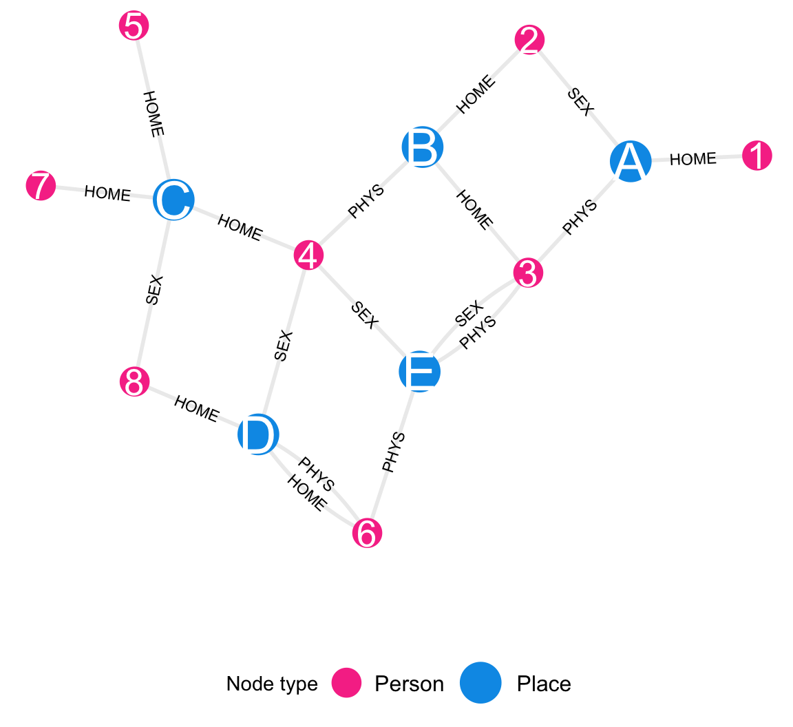
Figure B.1 is a data graph showing collected data. Community district nodes are shown in blue and survey participant nodes in pink. Each edge connects one community district with one survey participant. Three kinds of edges are shown – those that indicate either that the survey participant has a home in the community district, or that they attended a gathering with sexual contact or attended a gathering without sexual contact in the community district. For instance, Participant 3 has a home in Community District B, he attended a gathering with no sexual contact in Community District A, and he attended two gathering (one sexual and one non-sexual) in Community District E.
In this appendix, we outline an analysis of these data from the perspectives of: node characteristics, edge characteristics, local network structure, global network structure, and finally network dynamics.
We can examine patterns in the characteristics of participants as we usually do in descriptive analysis. In our example, these include variables age and vaccination status. We can tabulate and cross tabulate these variables to understand the composition of the study sample.
make_example_network_data() |>
  data.frame() |>
  dplyr::select(-label) |>
  gt::gt() |>
gt::tab_options(table.font.size =12, data_row.padding = gt::px(1))| Name | Node type | Age | Vax |
|---|---|---|---|
| Person 1 | Person | 18-25 | Yes |
| Person 2 | Person | 18-25 | No |
| Person 3 | Person | 18-25 | Yes |
| Person 4 | Person | 18-25 | No |
| Person 5 | Person | 26-50 | Yes |
| Person 6 | Person | 26-50 | No |
| Person 7 | Person | 26-50 | Yes |
| Person 8 | Person | 26-50 | No |
| Community a | Place | - | - |
| Community b | Place | - | - |
| Community c | Place | - | - |
| Community d | Place | - | - |
| Community e | Place | - | - |
We can also examine the characteristics of edges. These represent relations participants have with the communities in town. For instance, we can cross tablulate the “To” column with the “Relation” column to show the frequency of each kind of relation by community. This would help us to understand whether certain communities are popular destinations for physical or sexual contact, or even for residence.
make_example_network_data() |>
  dplyr::mutate(type, age) |>
  tidygraph::activate(edges) |>
  dplyr::mutate(from_name = tidygraph::.N()$name[from], to_name = tidygraph::.N()$name[to]) |>
  data.frame() |>
  dplyr::arrange(from, to) |>
  dplyr::transmute(From = from_name, To = to_name, Relation = relation) |>
  gt::gt() |>
gt::tab_options(table.font.size =12, data_row.padding = gt::px(1))| From | To | Relation |
|---|---|---|
| Person 1 | Community a | HOME |
| Person 2 | Community a | SEX |
| Person 2 | Community b | HOME |
| Person 3 | Community a | PHYS |
| Person 3 | Community b | HOME |
| Person 3 | Community e | SEX |
| Person 3 | Community e | PHYS |
| Person 4 | Community b | PHYS |
| Person 4 | Community c | HOME |
| Person 4 | Community d | SEX |
| Person 4 | Community e | SEX |
| Person 5 | Community c | HOME |
| Person 6 | Community d | PHYS |
| Person 6 | Community d | HOME |
| Person 6 | Community e | PHYS |
| Person 7 | Community c | HOME |
| Person 8 | Community c | SEX |
| Person 8 | Community d | HOME |
Examining local structure entails understanding how each node is related to the rest of the graph. We define spatial reach, social reach, spatial catchment, and social catchment.
Spatial reach is a person-node characteristic. It measures the number of relations to places the participant has. Note that we count relations and not places since one participant might have several relations with the same place.
make_reach_diagram_data() |>
  plot_reach_diagram() +
  theme_mpxnyc_blank(
                      plot.margin     = ggplot2::margin(40,20,40,20),
                      legend.position = "right"
) 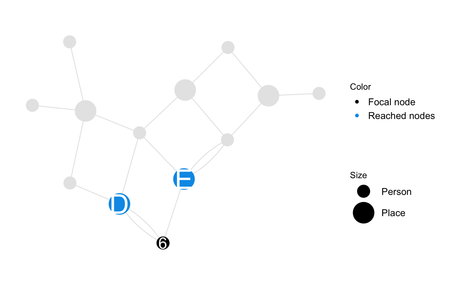
Spatial reach of person \(i\) is the number of relations person node \(i\) has with place nodes in the person-place graph.
\[ r_{i} = \sum_{ j }{ \Psi (i,j)} \]
Social catchment is a place-node characteristic which measures the number of relations with person nodes.
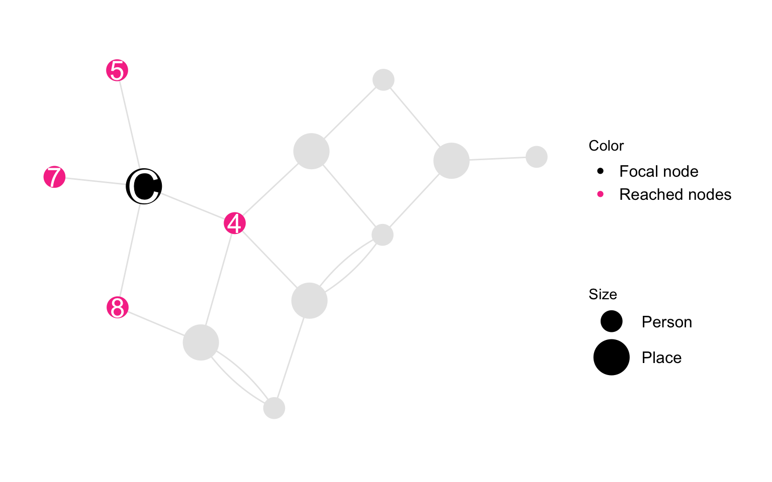
Social catchment of place \(j\) among subgroup \(A\) is defined as the number of connections the focal community district has with participants who belong to subgroup \(A \subset \mathscr{N}_P\). Social catchment of place \(j\) is defined as \(C_{j} = C_{j\rightarrow \mathscr{N}_P}\)
\[ C_{j\rightarrow A} = \sum_{i } { \Psi (i, j) A_i} \]
Spatial catchment is a place-node characteristic which measures the mutual influence between spatial untis as a result of relations with shared person nodes. It counts the number of minimal paths that link the focal node with other place nodes in the graph. Note that the number of paths that link two place nodes who are connected through a given person node is the product of the number of relations each place node has with the given person node.
make_reach_diagram_data(
  focal_node = "Community c",
  alter_nodes = c("Community d", "Community b", "Community e"),
  intermediate_nodes = c("Person 8", "Person 4")
  ) |>
  plot_reach_diagram(
   intermediate_color = "darkgrey"
  ) +
  theme_mpxnyc_blank(
                      plot.margin     = ggplot2::margin(40,20,40,20),
                      legend.position = "right"
) 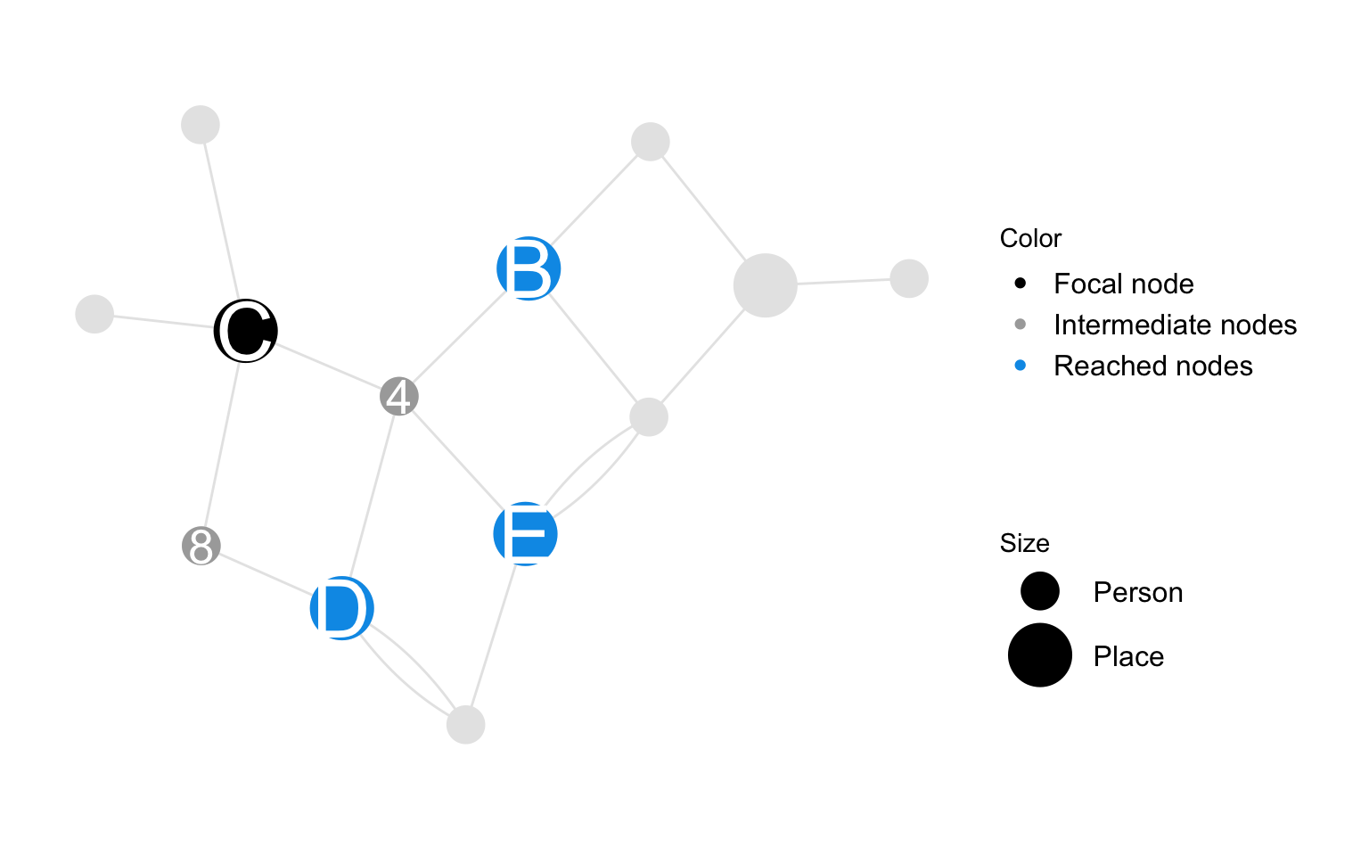
Spatial catchment of place \(j\) via subgroup \(A\) is defined as the strength of connection between place node \(j\) and other place nodes in the graph when we consider their shared relations with person nodes in subgroup \(A\). Strength of connection between two places \(j\) and \(k\) is defined as the number of relations place nodes \(j\) and \(k\) have with common person nodes which belong to subset \(A\). The spatial catchment of place \(j\) is defined as \(c_{i\rightarrow \mathscr{N}_P} = c_{i}\)
\[ c_{j\rightarrow A} = \sum_{i }\sum_{k }{ \Psi(i,j) \Psi(i,k)A_i} \\ \]
Measures of global structure quantify some aspect of the overall pattern of connection among the people and spaces connected by the data graph.
Spatial mixing is the extent to which person nodes with a given set of characteristics are connected to a common set of place nodes with person nodes with some other set of characteristics.
    base_color = "black"
    reached_color = "#009BE8"
    intermediate_color = "#C5EFFF"
    focal_color = "black"

        group_affiliation <- data.frame(
      name = c(paste("Person", 1:8)),
      group = c(
                "Group B",
                "Group A",
                "Group A",
                "Group B",
                "Group A",
                "Group B",
                "Group B",
                "Group A"
                )
    )

unmixed <- make_reach_diagram_data() |>
  tidygraph::mutate(type_color = NA) |>
  tidygraph::activate(nodes) |>
  tidygraph::left_join(group_affiliation) |>
  tidygraph::mutate(group = ifelse(type == "Place", "Place", group)) |>
  ggraph::ggraph(layout = "kk") +
    ggforce::geom_circle(ggplot2::aes(x0 = 0.5, y0 = 0, r = 2.3), data = data.frame(xmin = -3, xmax = 3, ymin = -1, ymax = 5), linewidth = 0, fill = "#FF99C5", alpha = 0.3) +
                  ggraph::geom_edge_fan(ggplot2::aes(color = type_color), show.legend = FALSE) +
                  ggraph::geom_node_point(ggplot2::aes( size = group), color = base_color) +
                  ggraph::geom_node_point(ggplot2::aes(color = age, size = group)) +
                  ggraph::geom_node_text(ggplot2::aes(label = label, size = group, filter = type == "Place"), color = "#FF99C5", show.legend = FALSE) +
                  ggplot2::scale_size_manual(name = "Size", values = c(7,7, 12), guide = "none") +
                scale_color_mpxnyc( name = "Age", option = "manual", na.value = base_color, values = c( "18-25" = "#F73C95",  "26-50" = "#009BE8", "Place" = "black"), na.translate = FALSE) +
                  ggraph::scale_edge_color_manual(values = c("black"), na.value = base_color) +
                  theme_mpxnyc_blank( legend.position = "bottom"
                                      ) +
  ggplot2::coord_fixed() +
  ggplot2::theme(
    legend.text = ggplot2::element_text(size = 20),
    legend.title = ggplot2::element_text(size = 20),
    legend.ticks = ggplot2::element_line(size = 20),
    legend.byrow = TRUE,
    legend.position = "right"
  ) +
ggplot2::guides(color = ggplot2::guide_legend(override.aes = list(size = 5))) # Adjust legend dot size base_color = "black"
reached_color = "#009BE8"
intermediate_color = "#C5EFFF"
focal_color = "black"
group_affiliation <- data.frame(
name = c(paste("Person", 1:8)),
group = c("Group B", "Group B", "Group B", "Group B", "Group A", "Group A", "Group A", "Group A")
)
mixed <- make_reach_diagram_data(
focal_node = "Community c",
alter_nodes = c("Community d", "Community b", "Community e"),
intermediate_nodes = c("Person 8", "Person 4")
) |>
tidygraph::mutate(type_color = NA) |>
tidygraph::activate(nodes) |>
tidygraph::left_join(group_affiliation) |>
tidygraph::mutate(group = ifelse(is.na(group), "Place", group)) |>
ggraph::ggraph(layout = "kk") +
ggforce::geom_circle(ggplot2::aes(x0 = 0.5, y0 = 0, r = 2.3), data = data.frame(xmin = -3, xmax = 3, ymin = -1, ymax = 5), linewidth = 0, fill = "#FF99C5", alpha = 0.3) +
ggraph::geom_edge_fan(ggplot2::aes(color = type_color), show.legend = FALSE) +
ggraph::geom_node_point(ggplot2::aes( size = group), color = base_color) +
ggraph::geom_node_point(ggplot2::aes(color = vax, size = group)) +
ggraph::geom_node_text(ggplot2::aes(label = label, size = group, filter = type == "Place"), color = "#FF99C5", show.legend = FALSE) +
ggplot2::scale_size_manual(name = "Size", values = c(7,7, 12), guide = "none") +
scale_color_mpxnyc(name = "Vax", option = "manual", na.value = base_color, values = c( "No" = "#F73C95", "Yes" = "#009BE8", "Place" = "black"), na.translate = FALSE) +
ggraph::scale_edge_color_manual(values = c("black"), na.value = base_color) +
theme_mpxnyc_blank( legend.position = "bottom"
) +
ggplot2::coord_fixed() +
ggplot2::theme(
legend.text = ggplot2::element_text(size = 20),
legend.title = ggplot2::element_text(size = 20),
legend.ticks = ggplot2::element_line(size = 20),
legend.byrow = FALSE,
legend.position = "right"
) +
ggplot2::guides(color = ggplot2::guide_legend(override.aes = list(size = 5, ncol = 1))) # Adjust legend dot size
cowplot::plot_grid(mixed, unmixed, rel_widths = c(1,1), nrow = 1)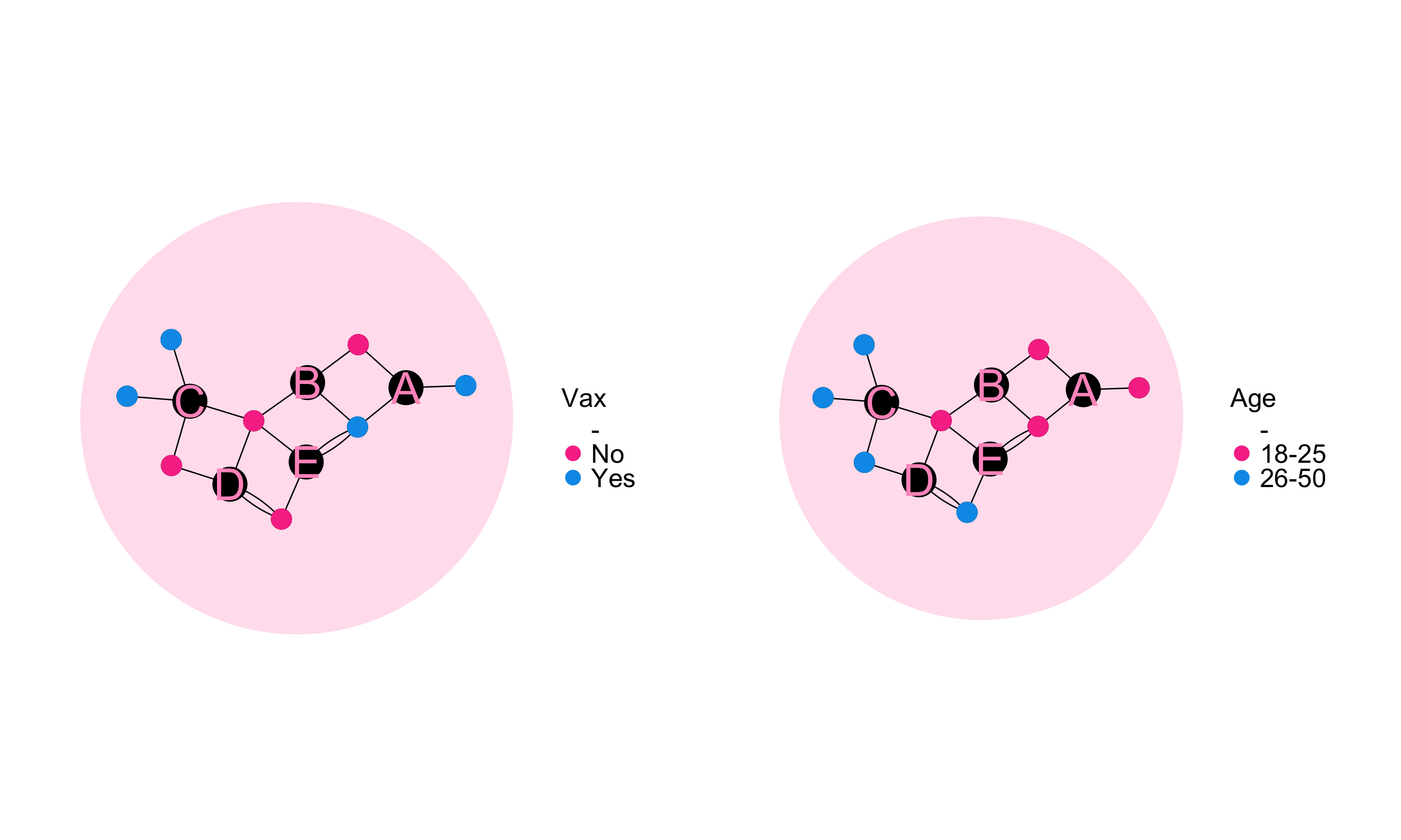
The spatial mixing coefficient from A to B quantifies the degree to which egos in group A preferentially live in or attend gatherings in community districts they are likely to encounter members of group B.
We define preference of group A for group B (for \(A, B \subset \mathscr{N}_p\)) as the average proportion of alters from group B among egos from group A.
\[ \Phi(A,B) = \frac{1}{|A|}\sum_{i \in A}{\frac{ R_{i \rightarrow B}}{R_i}} \]
The prevalence of group B is the size of the group divided by the total number of participants.
\[ \frac{|B|}{|\mathscr{N}_p|} \]
The spatial mixing coefficient is the ratio of preference to prevalence minus one.
\[ \phi(A,B) = \frac{|\mathscr{N}_p|}{|B|} \Phi(A,B) - 1 \]
Social connectedness is the extent to which all the person nodes are connected through a common set of space nodes. Equivalently, it is the extent to which space nodes are connected through a common set of person nodes.
    base_color = "black"
    reached_color = "#009BE8"
    intermediate_color = "black"
    focal_color = "black"

connectedness_connected <- make_reach_diagram_data(
  focal_node = "Community c",
  alter_nodes = c("Community d", "Community b", "Community e"),
  intermediate_nodes = c("Person 8", "Person 4")
  ) |>
  tidygraph::mutate(type_color = NA) |>
  tidygraph::activate(nodes) |>
  tidygraph::mutate(group = ifelse(runif(n = dplyr::n()) > 0.5, "Group A", "Group B")) |>
  tidygraph::mutate(group = ifelse(type == "Place", "Place", group)) |>
  ggraph::ggraph(layout = "kk") +
    ggforce::geom_circle(ggplot2::aes(x0 = 0.5, y0 = 0, r = 2.3), data = data.frame(xmin = -3, xmax = 3, ymin = -1, ymax = 5), linewidth = 0, fill = "#C5EFFF") +
  ggraph::geom_edge_fan(ggplot2::aes(color = type_color), show.legend = FALSE, edge_width = 1) +
  ggraph::geom_node_point(ggplot2::aes( size = group), color = base_color) +
  ggraph::geom_node_point(ggplot2::aes(color = group, size = group)) +
  ggraph::geom_node_text(ggplot2::aes(label = label, size = group,filter = type == "Place"), color = "#C5EFFF", show.legend = FALSE) +
  ggplot2::scale_size_manual(name = "Size", values = c(7,7, 12)) +
scale_color_mpxnyc(name = "Color", option = "manual", na.value = base_color, values = c( "Group A" = "black",  "Group B" = "black", "Place" = "black"), na.translate = FALSE) +
  ggraph::scale_edge_color_manual(values = c("black"), na.value = base_color) +
  theme_mpxnyc_blank(
                      plot.margin     = ggplot2::margin(20,20,20,20)
                      ) +
ggplot2::coord_fixed() base_color = grey(0.9,1)
base_color = "black"
reached_color = "#009BE8"
intermediate_color = "#C5EFFF"
focal_color = "black"
edge_hidden_data <- data.frame(
from = c(4,4,6, 2, 3, 6),
to = c(10, 13, 13, 10, 9, 12),
hidden = TRUE
)
connectedness_disconnected <- make_reach_diagram_data(
focal_node = "Community c",
alter_nodes = c("Community d", "Community b", "Community e"),
intermediate_nodes = c("Person 8", "Person 4")
) |>
tidygraph::mutate(type_color = NA) |>
tidygraph::left_join(edge_hidden_data) |>
tidygraph::mutate(hidden = ifelse(is.na(hidden), FALSE, hidden)) |>
tidygraph::activate(nodes) |>
tidygraph::mutate(group = ifelse(runif(n = dplyr::n()) > 0.5, "Group A", "Group B")) |>
tidygraph::mutate(group = ifelse(type == "Place", "Place", group)) |>
ggraph::ggraph(layout = "kk") +
ggforce::geom_circle(ggplot2::aes(x0 = 0.5, y0 = 0, r = 2.3), data = data.frame(xmin = -3, xmax = 3, ymin = -1, ymax = 5), linewidth = 0, fill = "#C5EFFF") +
ggplot2::coord_fixed() +
ggraph::geom_edge_fan(ggplot2::aes(color = type_color, filter = !hidden), show.legend = FALSE, edge_width = 1) +
ggraph::geom_node_point(ggplot2::aes( size = group), color = base_color) +
ggraph::geom_node_point(ggplot2::aes(color = group, size = group)) +
ggraph::geom_node_text(ggplot2::aes(label = label, size = group, filter = type == "Place"), color = "#C5EFFF", show.legend = FALSE) +
ggplot2::scale_size_manual(name = "Size", values = c(7,7, 12)) +
scale_color_mpxnyc(name = "Color", option = "manual", na.value = base_color, values = c( "Group A" = "black", "Group B" = "black", "Place" = "black"), na.translate = FALSE) +
ggraph::scale_edge_color_manual(values = c("black"), na.value = base_color) +
theme_mpxnyc_blank(
plot.margin = ggplot2::margin(20,20,20,20)
)
cowplot::plot_grid(connectedness_connected, connectedness_disconnected, rel_widths = c(1,1), nrow = 1)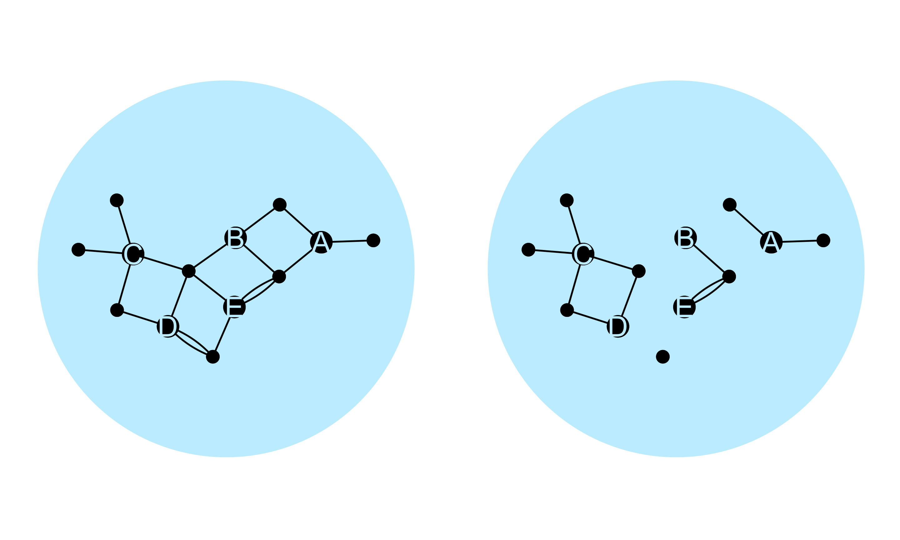
Proportion in largest connected component: In a given network, a connected component is a subset of nodes such that each node in the subset is reachable from any other node in the subset, and such that there are no nodes outside the subset which are reachable from a node inside it. By reachable, we mean possible to reach by tracing a path from one node to another over existing network ties. Say the size of the \(k^{th}\) connected component is \(C_k\) and the propoortion of nodes in that component is given by \(Q_k = C_k / n\). The proportion in the largest connected component is given by:
\[ \pi_Q = E[\max_k{Q_k}] \]
In studies which elicit participants’ primary residence along with other places they are related to, it may be of interest to understand the pattern of movement from home to related places and back again.
The movement matrix is a square matrix whose \(kl^{th}\) entry, \(m(k,l)\), is defined as the count of outings from home in community district \(k\) to a gathering in community district \(l\). Say \(d^H(i)\) is the home community district of participant \(i\).
\[ m(j,k) = \sum_i D(i,j) \sum_{k }( \Psi(i,k) - D(i,k) ) \]
The spatial concentration proportion \(c(k)\) quantifies the degree to which a community district is over-represented among destination community districts compared to home districts in the movement matrix. It is the difference of the margins of the movement matrix.
\[ c(k) = \frac{\sum_l{m(l,k)} - \sum_k{m(l,k)}}{\sum_{l,k}{m(l,k)}} \]
Lead author: Keletso Makofane, MPH, PhD. Editor: Nicholas Diamond, MPH. (Published: June 2025).
Acknowledgements: The analytic framework for this project developed over an extended period of time, beginning during my PhD dissertation at Harvard University under the supervision of Lisa Berkman, Eric Tchetgen Tchetgen, and a former mentor). In particular, the analysis borrows from the central paper in my dissertation, which shows how the wealth of non-coresident extended family members is protective against mortality. For publication-ready copies of the paper referenced below, which was accepted on 19 October 2023, please contact the editorial board of the American Journal of Epidemiology directly.
Makofane, K., Tchetgen Tchetgen, E. J., Bassett, M. T., Berkman, L. F. (Accepted 2023, final manuscript submitted January 2025). Networked wealth and mortality in the Agincourt Health and Demographic Surveillance System 2009 – 2018. American Journal of Epidemiology.
Social reach
Social reach is a person-node characteristic which measures the potential for interaction with other people through shared relations to places. It counts the number of minimal paths that link the focal node with other person nodes in the graph. Note that the number of paths that link two person nodes who are connected through a given place node is the product of the number of relations each person node has with the given place node.
Code
Let \(\psi(i,j)\) be the number of edges connecting person \(i\) and place \(j\) in the person-place graph. Social reach of person \(i\) among subgroup \(A\) is the number of person nodes in set \(A \subset \mathscr{N}_P\) that are connected to person node \(i\) through shared places. i.e. either because both nodes have a residence or gathering in at least one common community. Social reach of person \(i\) is defined as \(R_{i} = R_{i\rightarrow \mathscr{N}_P}\)
\[ R_{i\rightarrow A} = \sum_{j}{\sum_{k }{ \Psi(i,j) {\Psi(k,j)} A_k}} \]